Building Vector Search Into a SQL Query Engine

We added native ANN search to our DataFusion-based engine using USearch, Parquet, and SQLite — with adaptive filtering and got impressive results.

Today, if you want to add vector search to an application, you typically query a separate vector database that lives alongside your primary data store. Inspired by pgvector, we decided to bring vector search directly into our query engine, built on Apache DataFusion, and make vector search a first-class SQL operator.

In this post, we walk through the architecture, key design decisions, especially around filtered search, and benchmark results against LanceDB Cloud, who we consider the industry leader, on a 1.2 million row dataset.

What We Were Optimizing For

Vector search should be a SQL operator, not a separate service you query around.

Before diving in, it’s useful to understand our goals and design principles. Hotdata is primarily focused on latency rather than throughput, so we don’t have the same requirements as a many other databases.

We are primarily optimized for queries that process millions of records at a time, not full warehouse-scale scans. In practice, datasets are roughly 1–10 million vectors at 500–2000 dimensions, and we store data entirely in a single node. Since we’re not doing distributed vector search, managing what we keep in memory is our primary challenge. We do not assume all vectors fit into RAM, so we fall back to NVMe when necessary.

Finally, we target sub-100ms queries, even with filters applied. So we want to mix vector operations with standard filters like WHERE category=’nlp’ ORDER BY l2_distance() LIMIT 10 without any special syntax. This is important, and I’ll explain why below.

How We Store the Data

Hierarchical Navigable Small World (HNSW) is a state-of-the-art, graph-based algorithm for Approximate Nearest Neighbor (ANN) search used in vector databases for high-dimensional data retrieval.

When we ingest data, we build different indexes optimized for different access patterns. All three indexes share the same keys so we can easily toggle between stores. For example, key 0 in each store refers to the same record. This means that we are storage-heavy, but that’s a trade we’re willing to make.

The stores we have are:

USearch index: We use this to store the HNSW graph and raw vectors. This handles ANN search and lets us retrieve vectors directly by key. This is optimized for fast nearest neighbor search, but it doesn’t understand SQL predicates, which is why we use other layers for filtering.

SQLite: We store all scalar columns here. After we identify keys, we use SQLite to fetch the corresponding rows. Here we can get sub-millisecond lookups for fields like id, title, and metadata through a simple B-tree lookup. This works great with small datasets.

Parquet: We use Parquet to store the full dataset, including vectors, and to evaluate filters. It’s a columnar layout, and supports row group statistics, bloom filters, and page indexes. This lets us push down predicates and skip large portions of data. This works well for scanning and filtering, but not for point lookups.

So those are the building blocks. Now, let’s step through the different kinds of searches.

Unfiltered vector search

Lets analyze a simple vector search without any conditions or filters:

SELECT id, title, l2_distance(embedding, ARRAY[0.1, 0.2, ...]) AS dist
FROM my_table
ORDER BY dist ASC
LIMIT 10

When we execute it, the query goes through the following steps:

SQL query
  │
  ▼
Optimizer rewrites ORDER BY distance_fn(...) LIMIT k
  │
  ▼
USearch HNSW search(query_vector, k)
  │  returns: top-k keys + distances
  ▼
SQLite fetch_by_keys(keys)
  │  returns: scalar columns for those k rows
  ▼
Attach _distance column → result

We let USearch traverse the HNSW graph and return the k closest keys with their distances. On a million-row index, this usually runs in single-digit milliseconds. We then use SQLite to fetch the corresponding row data, such as id, title, and metadata, via primary key lookups.

Since there’s no filtering, we don’t touch Parquet at all.

Filtered vector search

Things get interesting when you introduce a WHERE clause. Consider this query:

SELECT id, l2_distance(embedding, ARRAY[...]) AS dist
FROM my_table
WHERE category = 'nlp'
ORDER BY dist ASC
LIMIT 10

The complicating part of this query is that the HNSW index is built over the entire dataset, but we only want results from the category = 'nlp' subset. The naive approach would have us first filter, then search, but that would require that we build a separate index per filter value. Instead, we use a two-phase strategy that decides the best execution path at runtime based on how selective the filter is.

Phase 1: Which rows match the filter?

Before we can search for nearest vectors, we need to know which rows match the WHERE clause. We do this with a lightweight Parquet scan that reads the key column and the columns referenced by the filter.

The filter predicate is pushed down to the Parquet reader, which can skip entire row groups and pages using Parquet’s built-in statistics, bloom filters, and page indexes.

1.2M rows in Parquet
        │
        ▼  scan _key + category only, push predicate down
        │
  ┌─────┴──────┐
  │ valid_keys │  →  { 42, 197, 1053, 8841, ... }
  │ (71K keys) │
  └─────┬──────┘
        │
        ▼  selectivity = 71K / 1.2M = 5.8%

This produces a set of keys that we need for the next phase and tells us both which rows to consider and how many.

Phase 2: Choosing between two paths

Once we know the total number of valid keys, we calculate the percentage of the keys we have on hand relative to the size of the table.

When we have high selectivity (> 5% of rows match), we pass the keys as a predicate callback to USearch’s filtered_search() which traverses the HNSW graph. It then returns top-k results and we fetch the result rows from SQLite.

                    selectivity?
                   /            \
            > 5%                  ≤ 5%
              │                     │
              ▼                     ▼
   HNSW filtered_search     index.get(key) for each valid_key
     with valid_keys           compute distances
     as predicate              maintain top-k heap
              │                     │
              ▼                     ▼
       SQLite fetch(k)         SQLite fetch(k)
              │                     │
              ▼                     ▼
           result                result

When we have low selectivity (≤ 5% of rows match), we use the USearch index as a key-value store: retrieve the vector for each valid key via index.get(), compute exact distances, maintain a top-k heap, and fetch result rows from SQLite.

This means we can avoid graph traversal completely and only do lookups. Which is very fast!

Benchmarks

To see how our approach compares, we benchmarked against LanceDB Cloud, a purpose-built vector database with HNSW support backed by the Lance columnar format. This is not an apples-to-apples comparison of equivalent architectures, but it’s good comparison point to understand how our approach stacks up.

Dataset: 1.2 million rows from the Sphere dataset. 768-dimensional embeddings (float64) plus scalar columns: id, url, title, sha, raw, filename.

Hotdata config: HNSW, M=16, ef_construction=128, ef_search=64, L2, F32 precision.

LanceDB config: IVF_HNSW_SQ, M=16, ef_construction=128, L2 (SQ = scalar quantization; the highest-recall HNSW variant available on their cloud).

Methodology: 5 random query vectors from the dataset. 1 cold run discarded, 3 warm runs averaged. All times are server-side execution time — LanceDB’s analyze_plan and our internal execution_time_ms .

Results

In our first comparison, Hotdata’s adaptive filtered search beats LanceDB across different filter types:

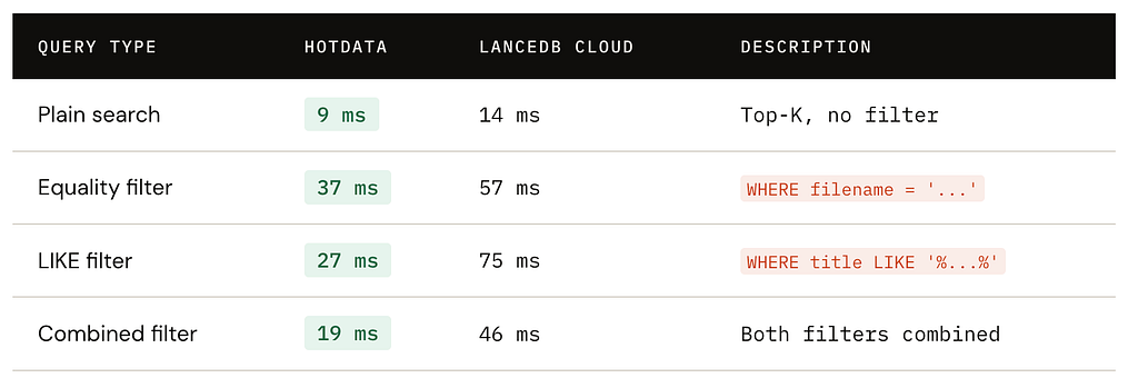
All queries return k=10.

Since Hotdata is focused on serving data, when comparing plain search, we see that performance scales well from k=10 to 500.

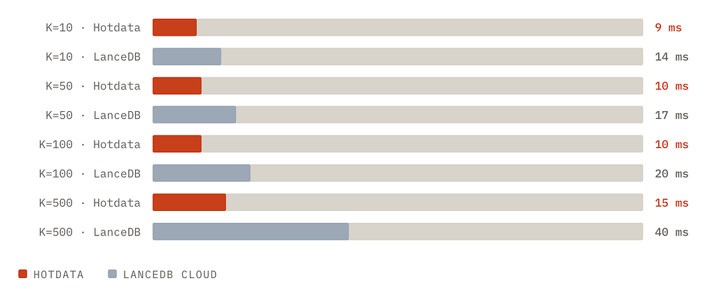
Hotdata’s latency is nearly flat from K=10 to K=500.

We were excited to see that this approach is proving to be quite fast and for our use-case we think we can refine it further. We’ll continue to post our findings.

What We Learned

The main takeaway is architectural: vector search and SQL dot not need to be fundamentally different systems. If you use a query engine that can treat ANN search as a natural extension of SQL, you can collapse layers of architecture.

From a developer experience standpoint, this is a major win.